The original dataset comprises Lidar tiles with classified ground and with XYZ ASCII format of this type :

13.83535621 42.12214528 401.940 32 2
13.83534713 42.12213870 401.870 28 2
13.83533818 42.12213222 401.670 33 2
13.83532879 42.12211645 401.950 30 1
13.83533763 42.12212258 401.630 28 2
13.83534682 42.12212933 401.830 29 2
13.83535625 42.12213609 402.250 25 1

2 processing methods are proposes. The first is more straightforward, it uses bash only. The second uses ArcGIS.

Method 1 : with bash, GDAL, LAStools

All the input tiles are compressed in zip format.

1- zip extraction :

for i in *.zip; do unzip $i -d .; done

The output is  xyz files, with classification as last field. 1 for unclassified, 2 for ground (see example above)

delete zip files with :
rm *.zip

2-extract only ground points from xyz files

awk '{if ($5==2) print $0}' input > output

for batch processing, see script “script_xyz2xyzground.sh”

3-convert xyz format to las format

las2las -i input -o output

4-interpolation in grid with points2grid

for i in *.las; do BASE=`basename $i .las`;points2grid -i $i -o OUTPUT/$BASE -r 0.00000707 --input_format las --output_format arc --mean --resolution 0.00001 --fill; done

5- convert asc format to tif

for i in *.asc; do BASE=`basename $i .asc`;gdal_translate -a_srs EPSG:4326 $i ${BASE}.tif;done

6- merge all tif tiles

gdal_merge.py -o MOSAIC/Marche_lidar_full_mosaic_4326.tif -co COMPRESS=DEFLATE -co BIGTIFF=YES -co TILED=YES -a_nodata 0 *.tif

Optional step : fill holes

for i in *.tif; do BASE=`basename $i ..tif`;gdal_fillnodata.py $i ${BASE}_filled.tif -co compress=deflate -co bigtiff=yes -co tiled=yes;done

Method 2 : with ArcGIS

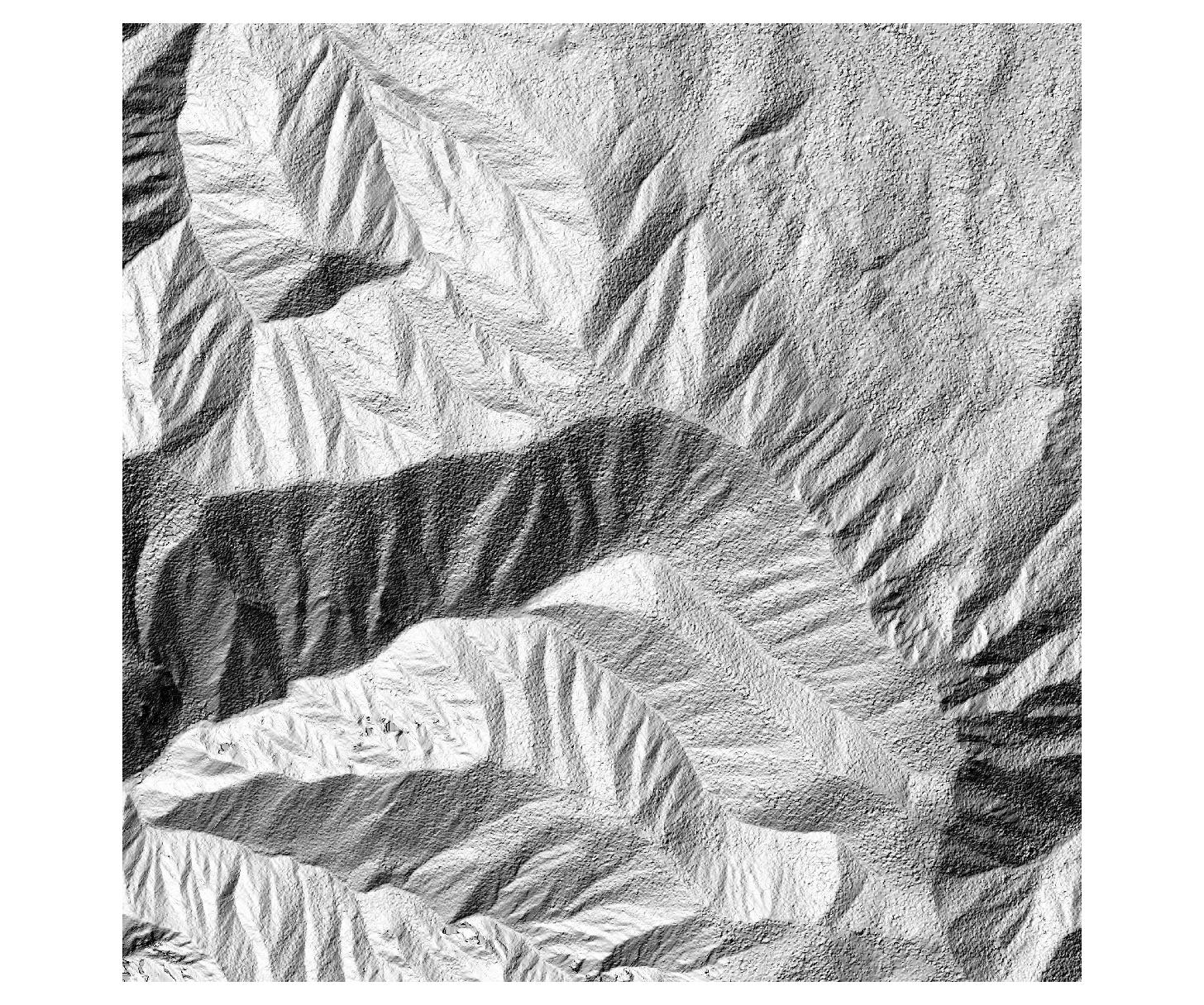
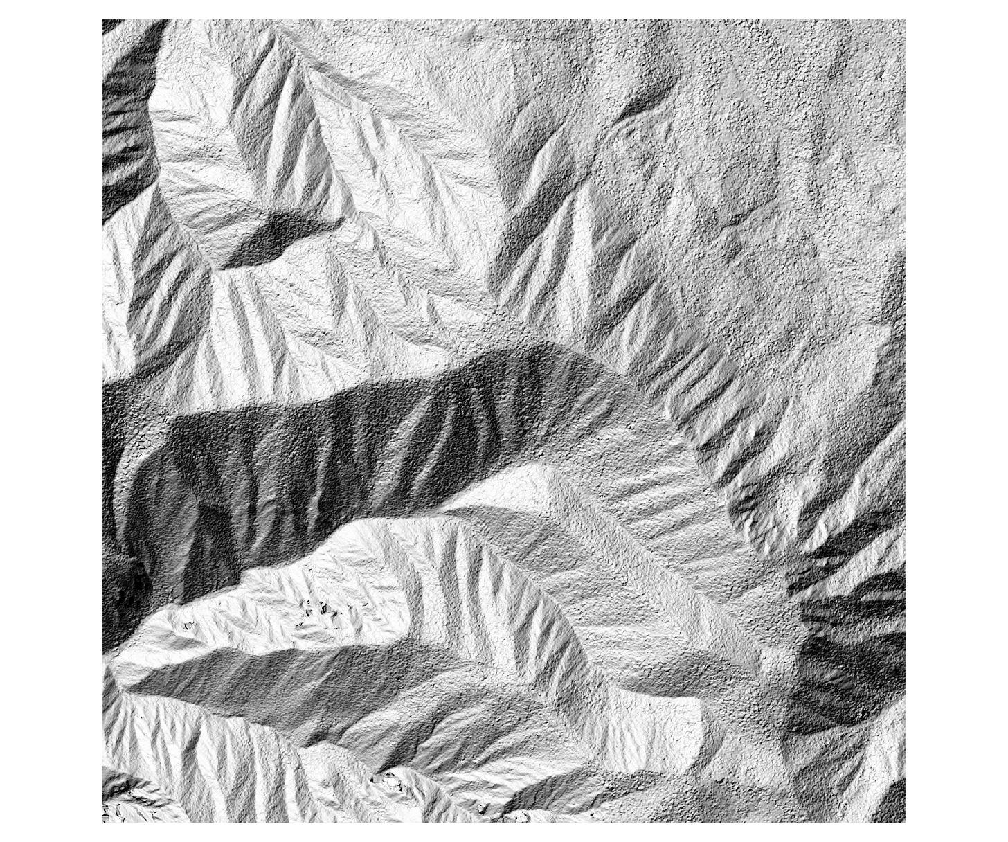
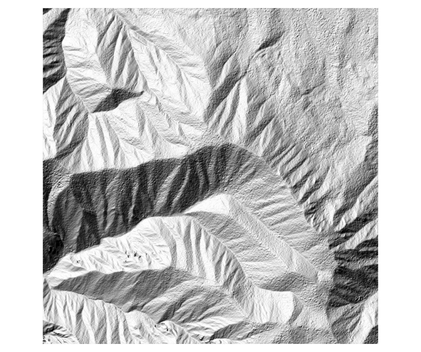
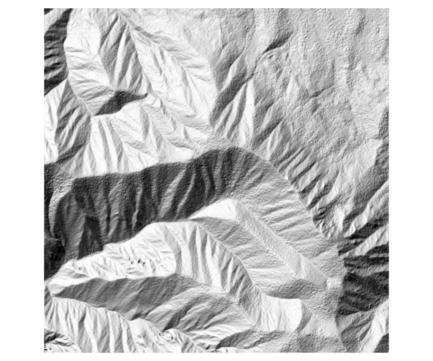
Toolbox of several small scripts for processing Lidar point cloud and generating DTMs

The original datasets are point clouds with ground already classified

Steps :

1 – extract only ground from the classified point cloud
This is done with awk. See description at this site https://sigeo.cerege.fr/?p=199

ex. of command for processing a file :
awk ‘{ if ( $5!=1 ) print $0 }’ input.xyz > output.xyz
to batch it in bash :
for i in *.xyz; do awk ‘{ if ( $5!=1 ) print $0 }’ input.xyz > output.xyz; done

2- Convert ASCII XYZ file to LAS
This is done with ArcGis using the txt2las tool of LAStools, but it can also be done with libLAS or PDAL
The script in the ArcGIS toolbox is used in a batch mode

3- Convert LAS files to LAS datasets
we created a small python script based on Arcpy that we use add to a Toolbox and use it in batch mode
see “convert_las2lasd.py”

4- Convert Las datasets to TIN
we created a small python script based on Arcpy that we use add to a Toolbox and use it in batch mode
see “convert_lasd2tin.py”

5- Convert Tin to raster
we created a small python script based on Arcpy that we use add to a Toolbox and use it in batch mode
see “convert_tin2raster.py”

The scripts of steps 2 to 5 are used from a ArcGIS Toolbox

Workflow pour filtrer les points du sol dans des données Lidar et créer un MNT

Ce workflow est un exemple de cas d’étude que nous avons eu à traiter, il est à adapter en fonction des données utilisées

Nous allons utiliser LibLAS, PDAL et Points2Grid

Données en entrée

Nous avons des nuages de points Lidar au format LAS, avec des coordonnées en WGS84 pour le X et Y, et en mètres pour le Z

Affichage des métadonnées (avec libLAS):

lasinfo input.las

Affichage des métadonnées (avecPDAL):

$ pdal info input.las

il faut vérifier si le système de coordonnées est définit, s’il y a un facteur d’échelle selon X, Y ou Z, et toutes autres informations

Supposons que le système de coordonnées n’est pas définit ou mal définit dans les métadonnées du LAS, cela va causer des problèmes dans la suite du traitement

Définition du système de coordonnées

Créer un fichier JSON pour le traitement PDAL, nommé par exemple “assign_scr.json” :

{
    "pipeline": [
        {
            "type" : "readers.las",
            "filename" : "input.las"
        },
        {
            "type" : "writers.las",
            "a_srs": "EPSG:4326",
            "filename" : "output.las"
        }
    ]
}

Puis lancer la commande:

pdal pipeline assign_scr.json

Maintenant la définition est correcte, mais il est préférable pour les interpolations et les traitements sur les MNT d’être en projection avec les mêmes unités en horizontal qu’en vertical, nous allons donc reprojeter en UTM

Reprojection

créer un pipeline JSON comme suit, nommé par exemple “reproject.json” :

{
  "pipeline":[
    { 
        "type":"writers.las", 
        "filename":"input.las" 
    }
    {
        "type":"filters.reprojection",
        "out_srs":"EPSG:32633"
    },
    {
      "type":"writers.las",
      "filename":"output.las"
    }
  ]
}

Puis lancer la commande:

pdal pipeline reproject.json

Il faut ensuite faire une classification sur les points

Classification du sol

créer un pipeline JSON comme suit, nommé par exemple “ground_classif.json” :

{
  "pipeline":[
    {
         "type":"filters.assign",
         "assignment":"Classification[:]=0"
    },
    {
         "type":"filters.elm"
    },
   {
         "type":"filters.outlier",
         "mean_k":8,
         "multiplier":3 
   },
   {
         "type":"filters.smrf",
         "ignore":"Classification[7:7]",
         "slope":0.2,
         "window":16,
         "threshold":0.45,
         "scalar":1.2
    },
    {
         "type":"filters.range",
         "limits":"Classification[2:2]"
     }
  ]
}

Ce pipeline est bien décrit dans les aides de PDAL, les étapes en sont les suivantes :

1. réassigner tous les points à la classe 0 car on suppose que la classification d’origine n’est pas bonne
2. utilisation de l’algo ELM pour assigner les points considérés comme du bruit à la classe 7
3. faire un filtrage statistique pour les points abbérants
4. utiliser le filtre SMRF sur les points restants pour classer les points
5. ne récupérer que les points classés comme ground

Puis lancer la commande:

pdal pipeline ground_classif.json

on récupère donc un fichier las ne contenant que les points classés comme sol (classe 2)

il est maintenant possible d’interpoler les points pour créer un MNT

Génération du MNT

l’interpolation peut se faire avec PDAL ou avec Points2Grid (outil utilisé par OpenTopography pour générer des MNT). L’implémentation de PDAL est basée sur celle de Points2Grid, donc au final c’est équivalent je pense.

La version de points2grid que nous utilisons est celle de développement ici

points2grid -i ground.las -o dtm.tif -r 1 --output_format grid --input_format las --interpolation_mode incore --idw --resolution 1 --fill --fill_window_size 5

pour des explications sur les paramètres taper : points2grid -h

Références:

• https://pdal.io/tutorial/ground-filters.html : filtrage sol sur PDAL, avec d’autres exemples encore sur ce site
• https://opentopography.org/otsoftware/points2grid : présentation générale de points2grid sur le site d’OpenTopography
• https://github.com/CRREL/points2grid/ : version de développement de points2grid